Note
Go to the end to download the full example code
Clip Volume Widget#
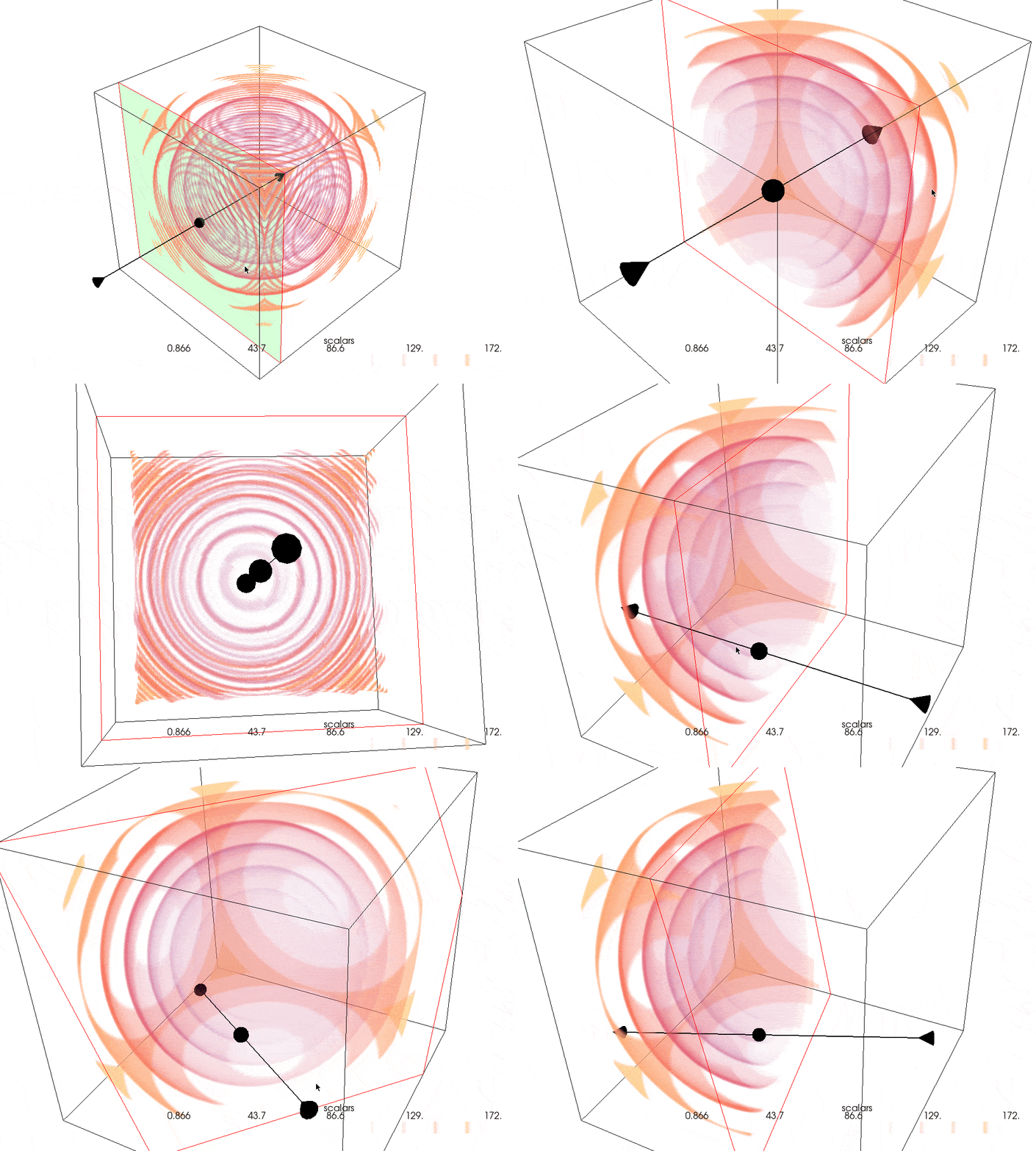
If you have a structured dataset like a pyvista.ImageData or
pyvista.RectilinearGrid, you can clip it using the
pyvista.Plotter.add_volume_clip_plane() widget to better see the internal
structure of the dataset.

Create the Dataset#
Create a dense pyvista.ImageData with dimensions (200, 200,
200) and set the active scalars to distance from the center of the grid.
import numpy as np

import pyvista as pv

grid = pv.ImageData(dimensions=(200, 200, 200))
grid['scalars'] = np.linalg.norm(grid.center - grid.points, axis=1)
grid
Generate the Opacity Array#
Create a banded opacity array such that our dataset shows “rings” at certain values. Have this increase such that higher values (values farther away from the center) are more opaque.
opacity = np.zeros(100)
opacity[::10] = np.geomspace(0.01, 0.75, 10)
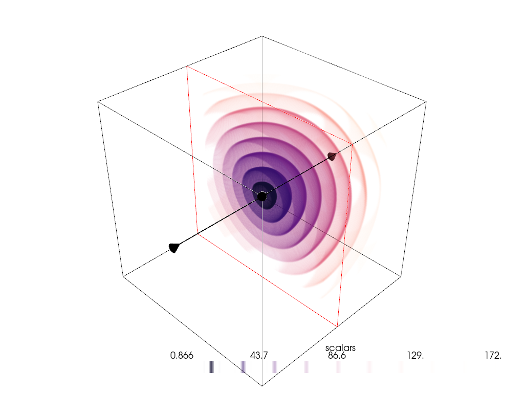
Plot a Single Clip Plane Dataset#
Plot the volume with a single clip plane.
Reverse the opacity array such that portions closer to the center are more opaque.

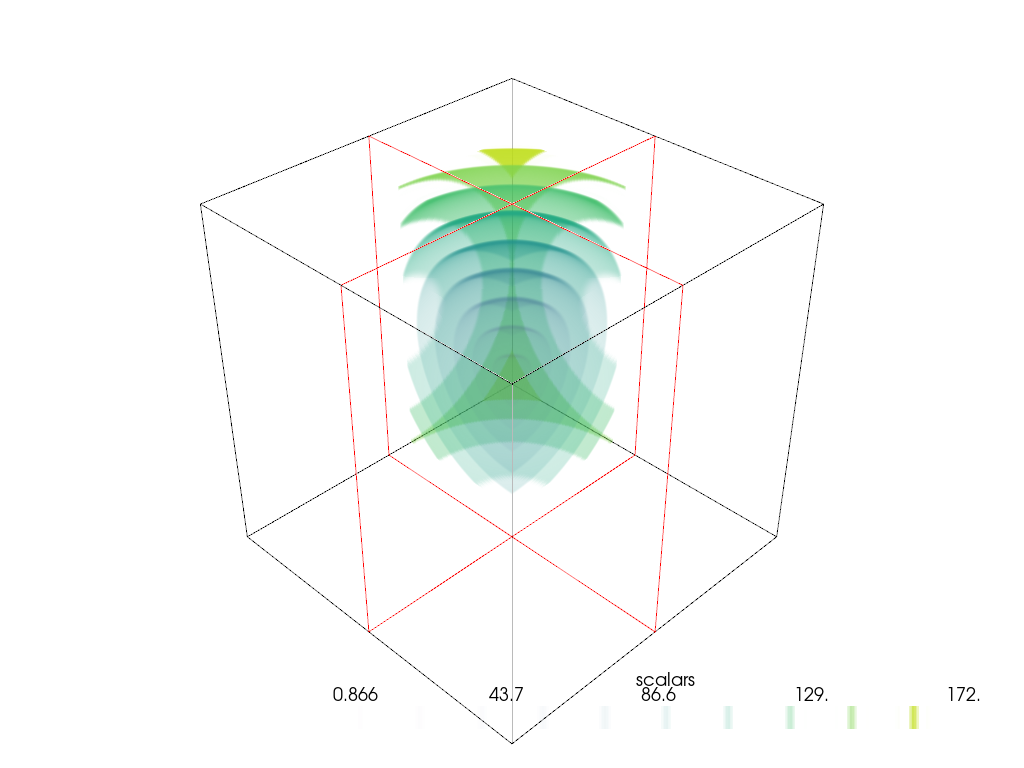
Plot Multiple Clip Planes#
Plot the dataset using the pyvista.Plotter.add_volume_clip_plane() with
the output from pyvista.Plotter.add_volume() Enable constant
interaction by setting the interaction_event to 'always'.
Disable the arrows to make the plot a bit clearer and flip the opacity array.
pl = pv.Plotter()
vol = pl.add_volume(grid, opacity=opacity)
vol.prop.interpolation_type = 'linear'
pl.add_volume_clip_plane(
    vol,
    normal='-x',
    interaction_event='always',
    normal_rotation=False,
)
pl.add_volume_clip_plane(
    vol,
    normal='-y',
    interaction_event='always',
    normal_rotation=False,
)
pl.show()

Total running time of the script: (0 minutes 15.335 seconds)