Plot a Magnetic Field

The following example demonstrates how PyVista can be used to plot a magnetic field.

This example relies on streamlines_from_source() to generate streamlines and add_volume() to plot the strength of the magnetic field.

This dataset was created from the Coil Field Lines example from the awesome magpylib library.

import numpy as np

import pyvista as pv
from pyvista import examples

Download the DataSet

Let’s first download the example dataset and show that it’s a pyvista.ImageData with the magnetic field stored as the 'B' array in point_data.

grid = examples.download_coil_magnetic_field()
grid.point_data

pyvista DataSetAttributes
Association     : POINT
Active Scalars  : B
Active Vectors  : B
Active Texture  : None
Active Normals  : None
Contains arrays :
    B                       float64    (531441, 3)          VECTORS

Create Coils

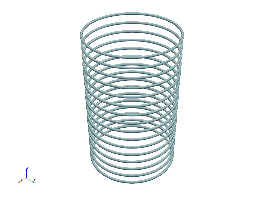
Create several hoops to represent the coil. This matches the geometry in the original example.

coils = []
for z in np.linspace(-8, 8, 16):
    coils.append(pv.Polygon((0, 0, z), radius=5, n_sides=100, fill=False))
coil_block = pv.MultiBlock(coils)
coil_block.plot(render_lines_as_tubes=True, line_width=10)

Compute and Plot Field Lines

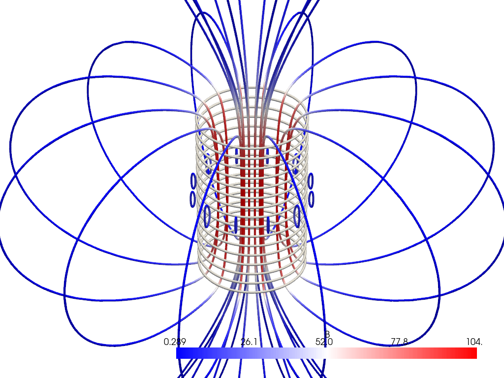
Next, let’s compute streamlines from the center of the coil to represent the direction of the magnetic force. For this, we can create a simple pyvista.Disc() and use that as the source of the streamlines.

seed = pv.Disc(inner=1, outer=5.4, r_res=2, c_res=12)
strl = grid.streamlines_from_source(
    seed,
    vectors='B',
    max_time=180,
    initial_step_length=0.1,
    integration_direction='both',
)

pl = pv.Plotter()
pl.add_mesh(
    strl.tube(radius=0.1),
    cmap='bwr',
    ambient=0.2,
)
pl.add_mesh(coil_block, render_lines_as_tubes=True, line_width=5, color='w')
pl.camera.zoom(3)
pl.show()

Plot the Magnet Field Strength

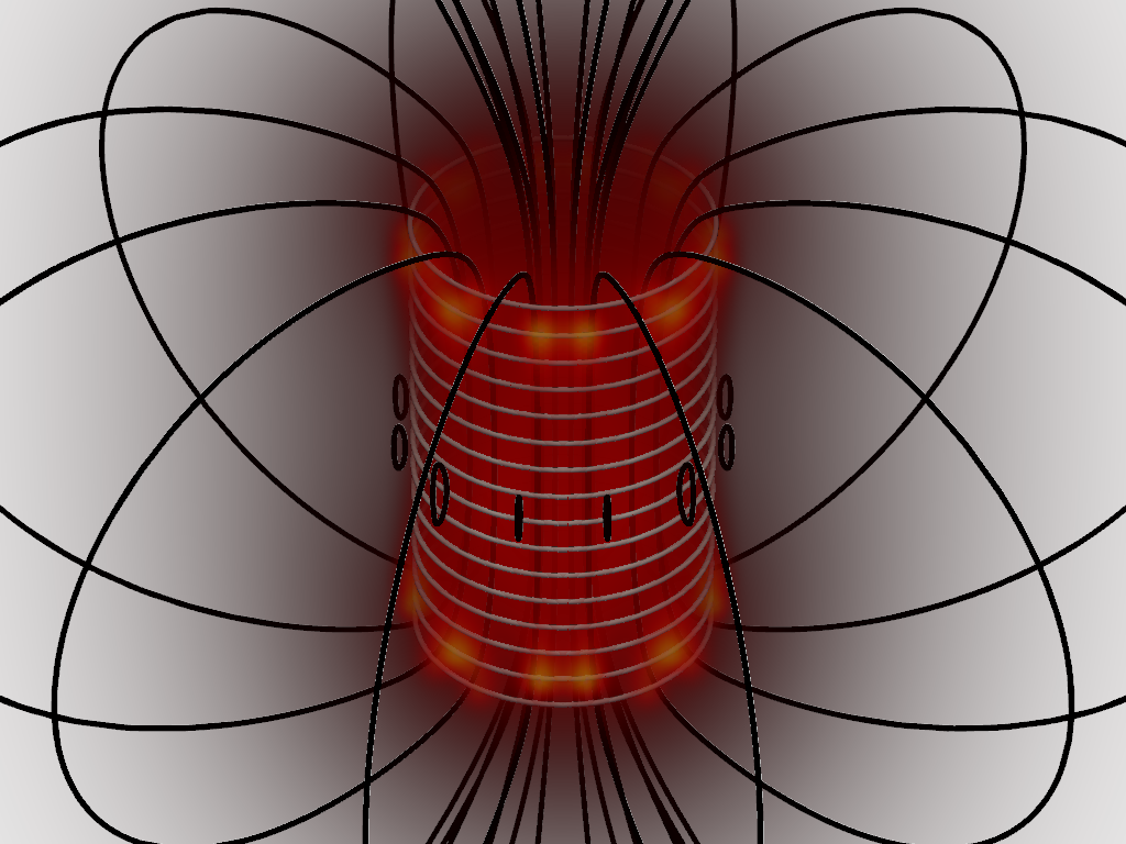
Finally, let’s bring this all together by plotting the magnetic field strength while also plotting the streamlines and the coil.

# Take the norm of the magnetic field
scalars = np.linalg.norm(grid['B'], axis=1)

# Customize the opacity to make it easier to visualize the strength of the
# field nearby the coil
opacity = 1 - np.geomspace(1.0, 0.05, 10)

# Add this all to the plotter
pl = pv.Plotter()
pl.add_mesh(
    strl.tube(radius=0.1),
    color='black',
)
pl.add_mesh(coil_block, render_lines_as_tubes=True, line_width=5, color='w')
vol = pl.add_volume(
    grid,
    scalars=scalars,
    opacity=opacity,
    cmap='hot',
    show_scalar_bar=False,
)
vol.prop.interpolation_type = 'linear'
pl.camera.zoom(5)
pl.show()