Note
Go to the end to download the full example code
Plot with Opacity#
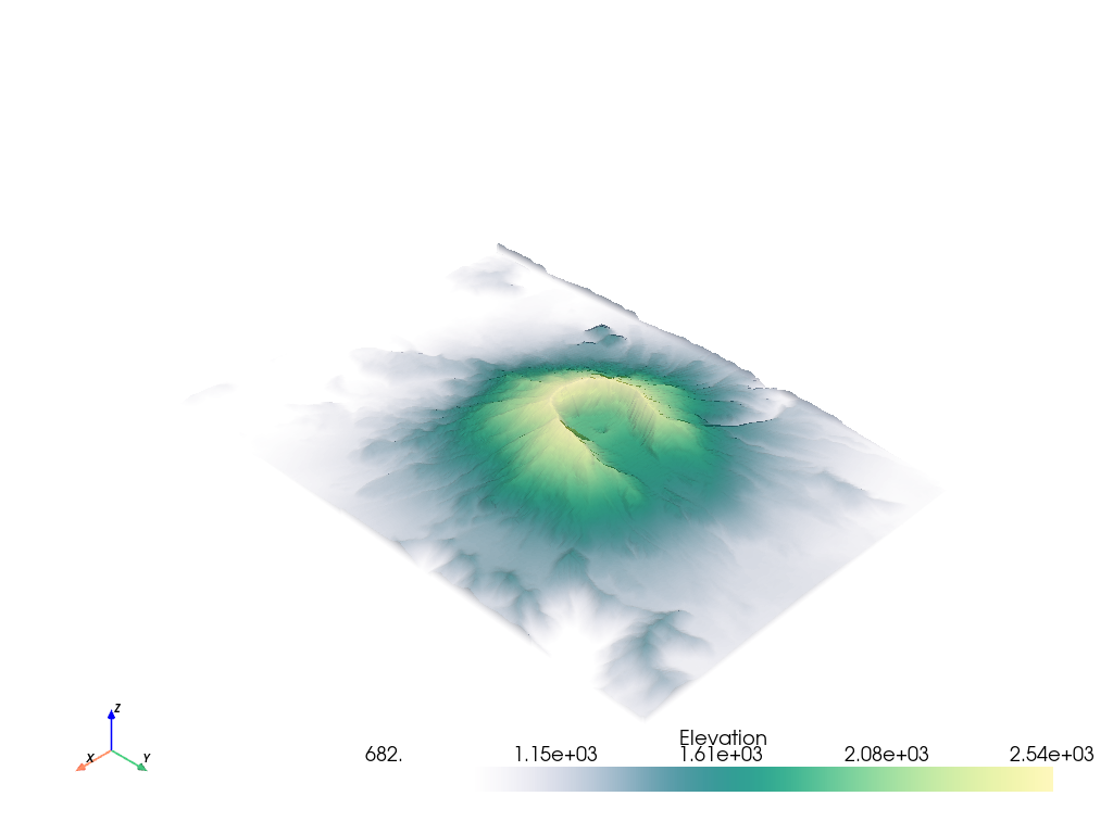
Plot a mesh’s scalar array with an opacity transfer function or opacity mapping based on a scalar array.
import pyvista as pv
from pyvista import examples

# Load St Helens DEM and warp the topography
image = examples.download_st_helens()
mesh = image.warp_by_scalar()
Global Value#
You can also apply a global opacity value to the mesh by passing a single float between 0 and 1 which would enable you to see objects behind the mesh:
p = pv.Plotter()
p.add_mesh(
    image.contour(),
    line_width=5,
)
p.add_mesh(mesh, opacity=0.85, color=True)
p.show()
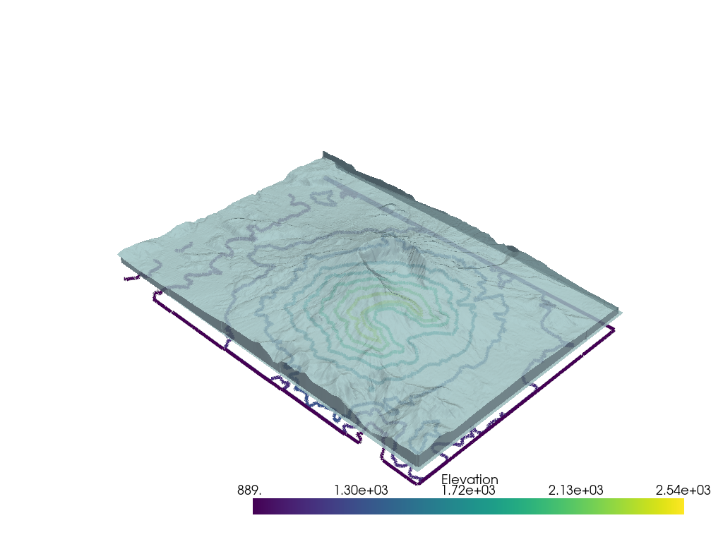
Note that you can specify use_transparency=True to convert opacities to
transparencies in any of the following examples.
Transfer Functions#
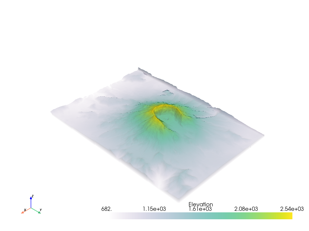
It’s possible to apply an opacity mapping to any scalar array plotted. You can specify either a single static value to make the mesh transparent on all cells, or use a transfer function where the scalar array plotted is mapped to the opacity. We have several predefined transfer functions.
Opacity transfer functions are:
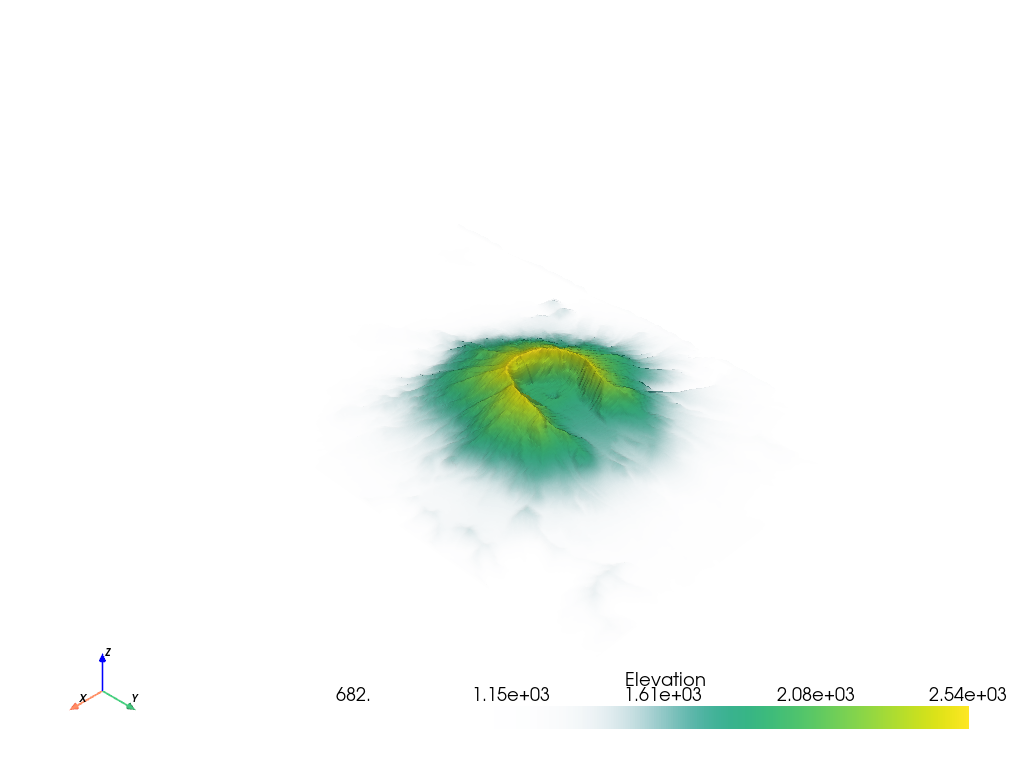
'linear': linearly vary (increase) opacity across the plotted scalar range from low to high'linear_r': linearly vary (increase) opacity across the plotted scalar range from high to low'geom': on a log scale, vary (increase) opacity across the plotted scalar range from low to high'geom_r': on a log scale, vary (increase) opacity across the plotted scalar range from high to low'sigmoid': vary (increase) opacity on a sigmoidal s-curve across the plotted scalar range from low to high'sigmoid_r': vary (increase) opacity on a sigmoidal s-curve across the plotted scalar range from high to low
# Show the linear opacity transfer function
mesh.plot(opacity="linear")
# Show the sigmoid opacity transfer function
mesh.plot(opacity="sigmoid")
It’s also possible to use your own transfer function that will be linearly mapped to the scalar array plotted. For example, we can create an opacity mapping as:
opacity = [0, 0.2, 0.9, 0.6, 0.3]
When given a minimized opacity mapping like that above, PyVista interpolates
it across a range of how many colors are shown when mapping the scalars.
If scipy is available, then a quadratic interpolation is used -
otherwise, a simple linear interpolation is used.
Curious what that opacity transfer function looks like? You can fetch it:
# Have PyVista interpolate the transfer function
tf = pv.opacity_transfer_function(opacity, 256).astype(float) / 255.0

import matplotlib.pyplot as plt

plt.plot(tf)
plt.title('My Interpolated Opacity Transfer Function')
plt.ylabel('Opacity')
plt.xlabel('Index along scalar mapping')
plt.show()
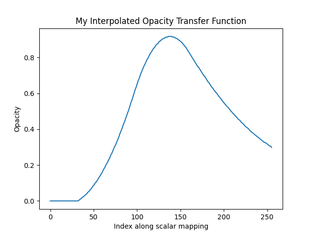
That opacity mapping will have an opacity of 0.0 at the minimum scalar range, a value or 0.9 at the middle of the scalar range, and a value of 0.3 at the maximum of the scalar range:
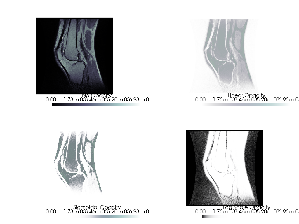
Opacity mapping is often useful when plotting DICOM images. For example, download the sample knee DICOM image:
knee = examples.download_knee()
And here we inspect the DICOM image with a few different opacity mappings:
p = pv.Plotter(shape=(2, 2), border=False)

p.add_mesh(knee, cmap="bone", scalar_bar_args={'title': "No Opacity"})
p.view_xy()

p.subplot(0, 1)
p.add_mesh(knee, cmap="bone", opacity="linear", scalar_bar_args={'title': "Linear Opacity"})
p.view_xy()

p.subplot(1, 0)
p.add_mesh(knee, cmap="bone", opacity="sigmoid", scalar_bar_args={'title': "Sigmoidal Opacity"})
p.view_xy()

p.subplot(1, 1)
p.add_mesh(knee, cmap="bone", opacity="geom_r", scalar_bar_args={'title': "Log Scale Opacity"})
p.view_xy()

p.show()
Opacity by Array#
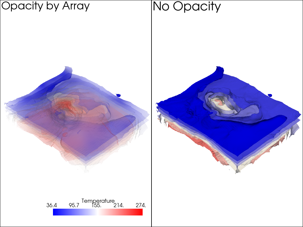
You can also use a scalar array associated with the mesh to give each cell its own opacity/transparency value derived from a scalar field. For example, an uncertainty array from a modelling result could be used to hide regions of a mesh that are uncertain and highlight regions that are well resolved.
The following is a demonstration of plotting a mesh with colored values and using a second array to control the transparency of the mesh
model = examples.download_model_with_variance()
contours = model.contour(10, scalars='Temperature')
contours.array_names
['Temperature', 'Temperature_var']
Make sure to flag use_transparency=True since we want areas of high
variance to have high transparency.
Also, since the opacity array must be between 0 and 1, we normalize the temperature variance array by the maximum value. That way high variance will be completely transparent.
contours['Temperature_var'] /= contours['Temperature_var'].max()

p = pv.Plotter(shape=(1, 2))

p.subplot(0, 0)
p.add_text('Opacity by Array')
p.add_mesh(
    contours.copy(),
    scalars='Temperature',
    opacity='Temperature_var',
    use_transparency=True,
    cmap='bwr',
)

p.subplot(0, 1)
p.add_text('No Opacity')
p.add_mesh(contours, scalars='Temperature', cmap='bwr')
p.show()
Total running time of the script: (0 minutes 25.701 seconds)