Note
Go to the end to download the full example code
Customize Scalar Bars#
Walk through of all the different capabilities of scalar bars and how a user can customize scalar bars.
import pyvista as pv
from pyvista import examples
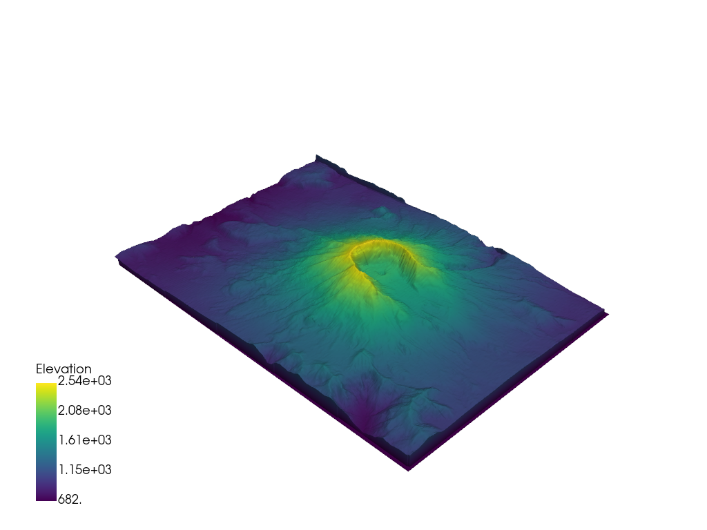
By default, when plotting a dataset with a scalar array, a scalar bar for that
array is added. To turn off this behavior, a user could specify
show_scalar_bar=False when calling .add_mesh(). Let’s start with a
sample dataset provide via PyVista to demonstrate the default behavior of
scalar bar plotting:
# Load St Helens DEM and warp the topography
mesh = examples.download_st_helens().warp_by_scalar()

# First a default plot with jet colormap
p = pv.Plotter()
# Add the data, use active scalar for coloring, and show the scalar bar
p.add_mesh(mesh)
# Display the scene
p.show()

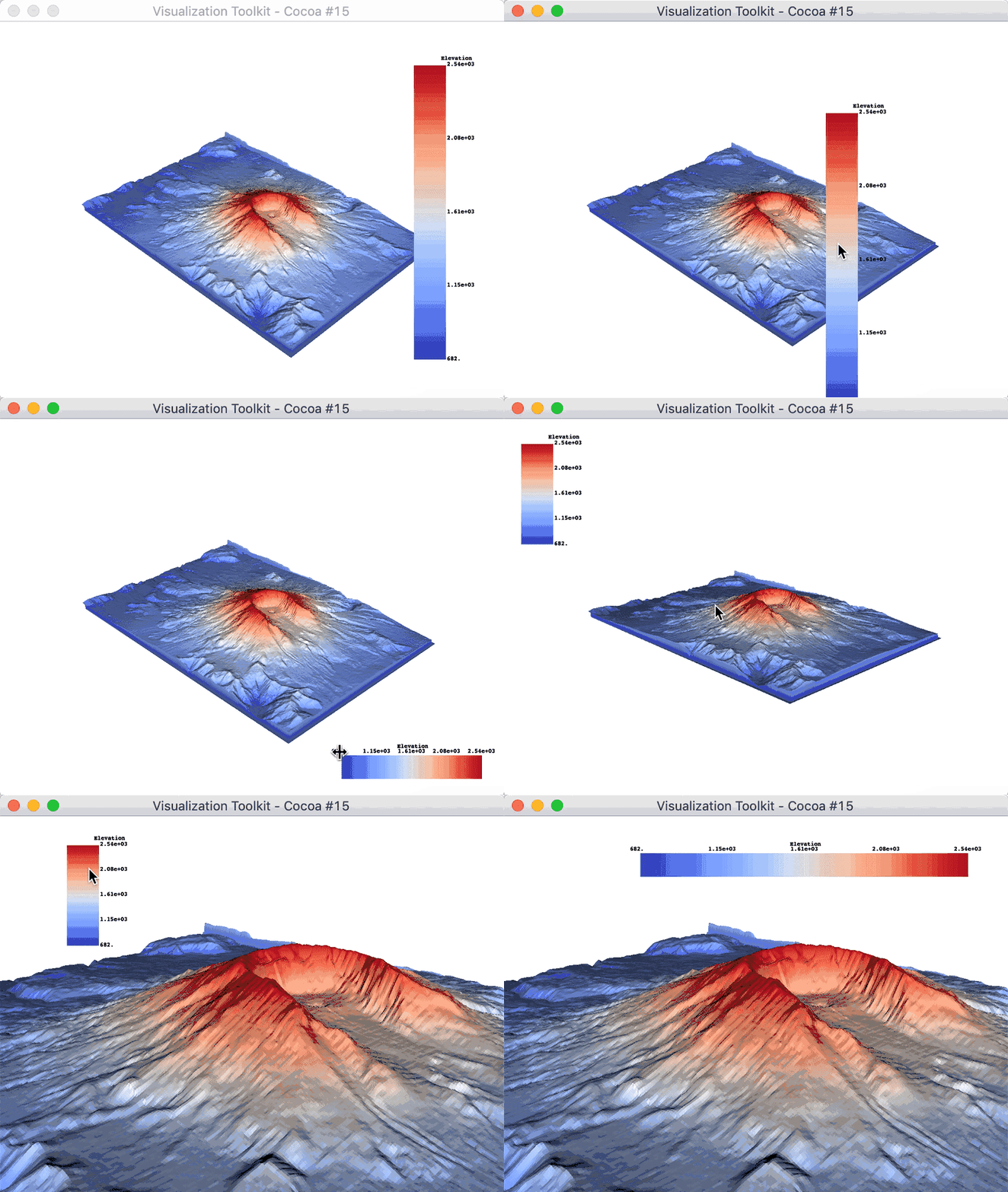
We could also plot the scene with an interactive scalar bar to move around
and place where we like by specifying passing keyword arguments to control
the scalar bar via the scalar_bar_args parameter in
pyvista.Plotter.add_mesh(). The keyword arguments to control the
scalar bar are defined in pyvista.Plotter.add_scalar_bar().
# create dictionary of parameters to control scalar bar
sargs = dict(interactive=True)  # Simply make the bar interactive

p = pv.Plotter(notebook=False)  # If in IPython, be sure to show the scene
p.add_mesh(mesh, scalar_bar_args=sargs)
p.show()
# Remove from plotters so output is not produced in docs
pv.plotting.plotter._ALL_PLOTTERS.clear()

Or manually define the scalar bar’s location:

The text properties of the scalar bar can also be controlled:

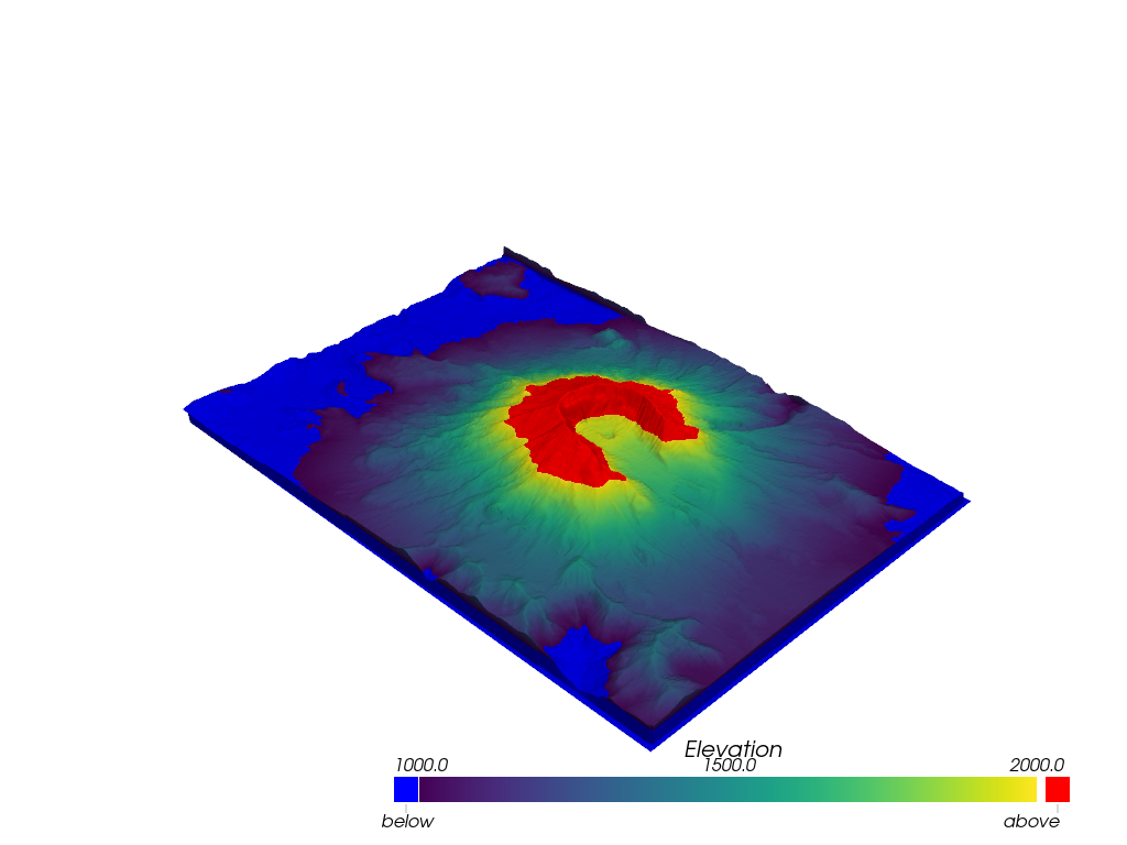
Labelling values outside of the scalar range
p = pv.Plotter()
p.add_mesh(mesh, clim=[1000, 2000], below_color='blue', above_color='red', scalar_bar_args=sargs)
p.show()

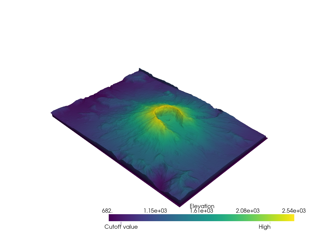
Annotate values of interest using a dictionary. The key of the dictionary must be the value to annotate, and the value must be the string label.
# Make a dictionary for the annotations
annotations = {
    2300: "High",
    805.3: "Cutoff value",
}

p = pv.Plotter()
p.add_mesh(mesh, scalars='Elevation', annotations=annotations)
p.show()

Total running time of the script: (0 minutes 11.519 seconds)